Differentiable color grading
from tinycio import ColorImage, ColorCorrection, LookupTable
from tinycio.util import progress_bar

im_src = ColorImage.load('my/source.exr', 'SRGB_LIN')
im_tgt = ColorImage.load('my/target.exr', 'SRGB_LIN')
im_src_cc = im_src.to_color_space('ACESCC')
im_tgt_cc = im_tgt.to_color_space('ACESCC')

# Option 1
auto_lut = LookupTable.get_linear(size = 64)
auto_lut.fit_to_image(im_src, im_tgt, context = progress_bar)
auto_lut.save('my/auto_lut.cube')
im_src.lut(auto_lut).to_color_space('SRGB').save('my/result1.png')

# Option 2
auto_cc = ColorCorrection()
auto_cc.fit_to_image(im_src_cc, im_tgt_cc, context = progress_bar)
auto_cc.save('my/auto_cc.toml')
im_src.correct(auto_cc).to_color_space('SRGB').save('my/result2.png')
What this is doing
I would like to call it “differentiable color grading” – and if that doesn’t catch on, I propose “autograde.” There is no artificial neural network involed in the process. In fact, no neural network is needed to perform gradient descent directly on a target. We have two such targets and, as it turns out, both are adequate choices with a relatively simple loss calculation.
The first approach creates a color grading 3D LUT by aligning the appearance of a source image to that of a target image. The second does the same, only by optimizing color correction settings instead of directly optimizing a 3D LUT.
Let’s try to undo a simple transformation by fitting a LUT to the original image as target.
cc = ColorCorrection()
cc.set_color_filter(0.6, 0.25)
cc.set_contrast(0.6)
cc.set_exposure_bias(0.8)
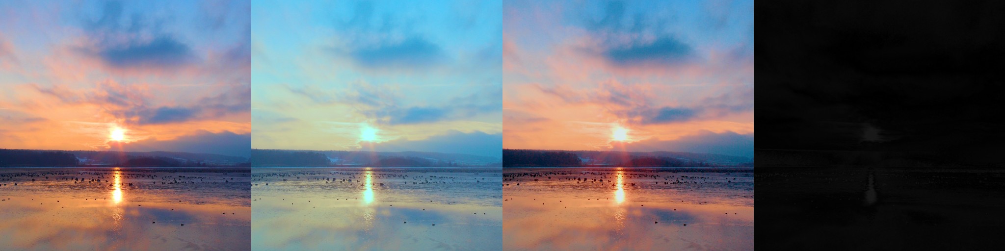
Fig. 10 LookupTable optimization: source image, transformation, recovery, error (photograph by saso ucitelj [2])
Keep in mind that we can’t rely on pixel-for-pixel comparisons. So, if we push it too far, this approach obviously breaks.
cc = ColorCorrection()
cc.set_color_filter(0.6, 0.25)
cc.set_saturation(1.4)
cc.set_shadow_color(0.3, 0.5)
cc.set_hue_delta(0.2)
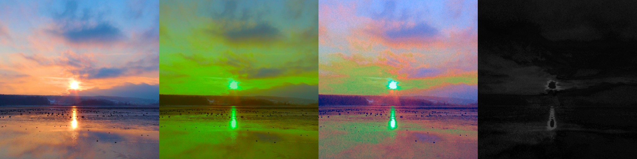
Fig. 11 LookupTable optimization: source image, transformation, recovery, error
Optimizing the color correction controls instead, on the other hand, is significantly more resilient.
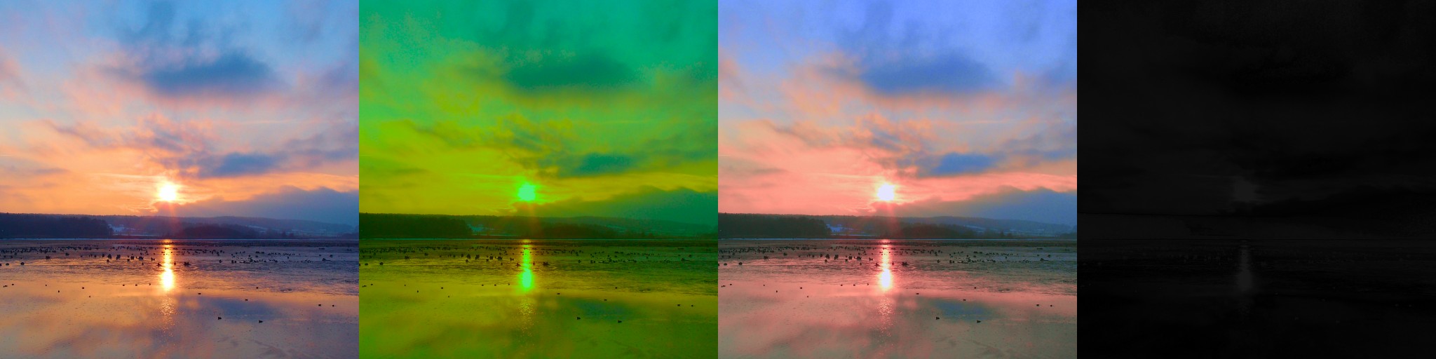
Fig. 12 ColorCorrection optimization: source image, transformation, recovery, error
LUT: the brute-force approach
Optimizing the CUBE LUT directly is straighforward:
# Create a linear lookup table (output matches input one-to-one)
auto_lut = LookupTable.get_linear(size = 64)

# Gradient descent on LUT, with source and target images to evaluate loss
auto_lut.fit_to_image(im_src, im_tgt, context = progress_bar)

# Save the LUT to disk when completed
auto_lut.save('my/auto_lut.cube')

# Apply the LUT to the source image and save it
im_src.lut(auto_lut).save('my/result1.png')
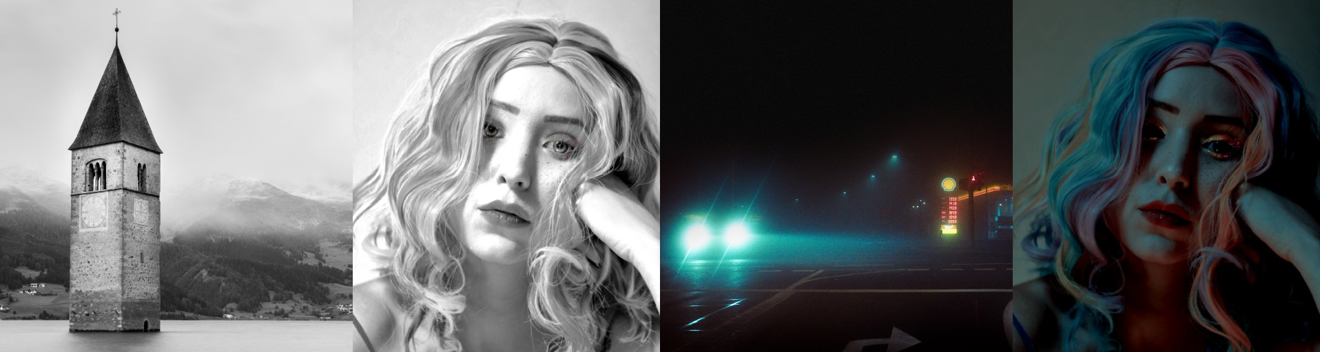
Fig. 13 LookupTable optimization
(photographs by Bruno Kraler [6] and Pepe Caspers [7] respectively)
Settings: a little finesse
The second option is to give autograd the keys and let it drive color correction:
# Create a new ColorCorrection object
auto_cc = ColorCorrection()

# Gradient descent on settings, with source and target images to evaluate loss
auto_cc.fit_to_image(im_src, im_tgt, context = progress_bar)

# Save the settings to disk when completed
auto_cc.save('my/auto_cc.toml')

# Apply the color correction to the source and save it
im_src.correct(auto_cc).save('my/result2.png')

# Print out the settings
auto_cc.info()

# Prints e.g.:

# CC DESCRIPTION:
# ===============
# CLASS            ColorCorrection
# EXPOSURE BIAS    -0.17404550313949585
# COLOR FILTER     [0.808641   0.81534934 0.9074043 ]
# HUE DELTA        0.0
# SATURATION       1.5330744981765747
# CONTRAST         1.2529858350753784
# SHADOW COLOR     [0.         0.         0.22277994]
# MIDTONE COLOR    [0.16701505 0.16309454 0.        ]
# HIGHLIGHT COLOR  [0.         0.         0.09913802]
# SHADOW OFFSET    -0.2189391404390335
# MIDTONE OFFSET   0.14226016402244568
# HIGHLIGHT OFFSET 0.007211057469248772

# And if you like:
auto_cc.bake_lut(size = 64).save('my/auto_lut.cube')
This has a few distinct advantages:
You can further alter the settings after optimization.
You can save the settings as a tiny toml file and reuse them.
You can still later bake a LUT of any size and in any color space you prefer.
It also overall seems to generate more plausible results.
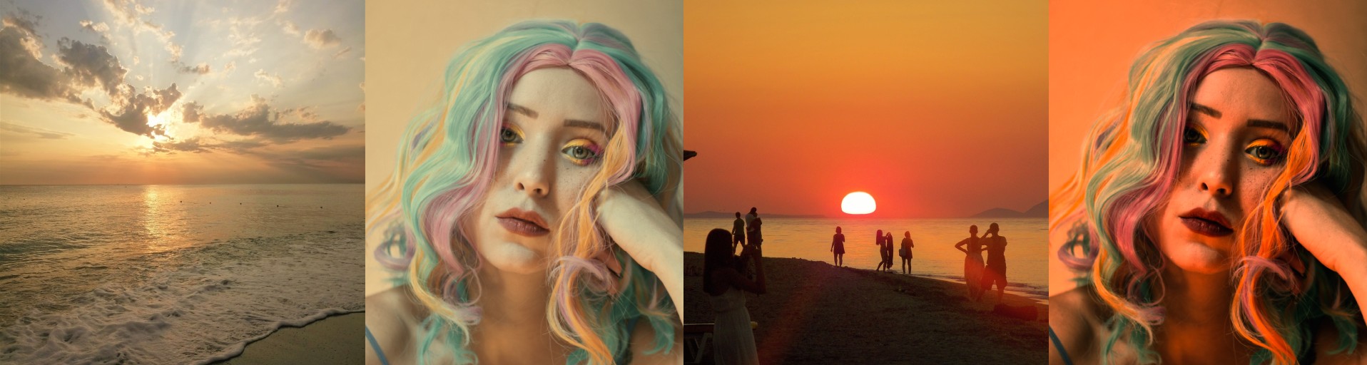
Fig. 14 ColorCorrection optimization
(photographs by saso ucitelj [2])
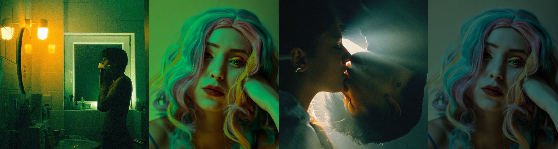
Fig. 15 ColorCorrection optimization
(photographs by Diep Minh Chien Tran [3])
Limitations
One application for this kind of image processing is as a tool to facilitate compositing. The obvious disadvantage of doing this with no ANN, however, is that the optimizer is semantically unaware of the scene; we are treating images as mere buckets of color. As there’s no image segmentation involved, this technique is probably best suited for, in some sense, “proposing a color palette” rather than trying to meaningfully match scene features.
What’s worse is that (directly) fitted LUTs will likely not generalize well at all, making them essentially one-time use. The response curves produced by a fitted LUT are not guaranteed to be monotonic, or even to make any sense at all once removed from the specific colors optimized and applied to a different image. For example, adding more to the red channel may produce much less red - not for some nuanced reason actually modeling something, but just because. The optimizer was perhaps not made aware those colors even exist.
A few problem cases are illustrated below.
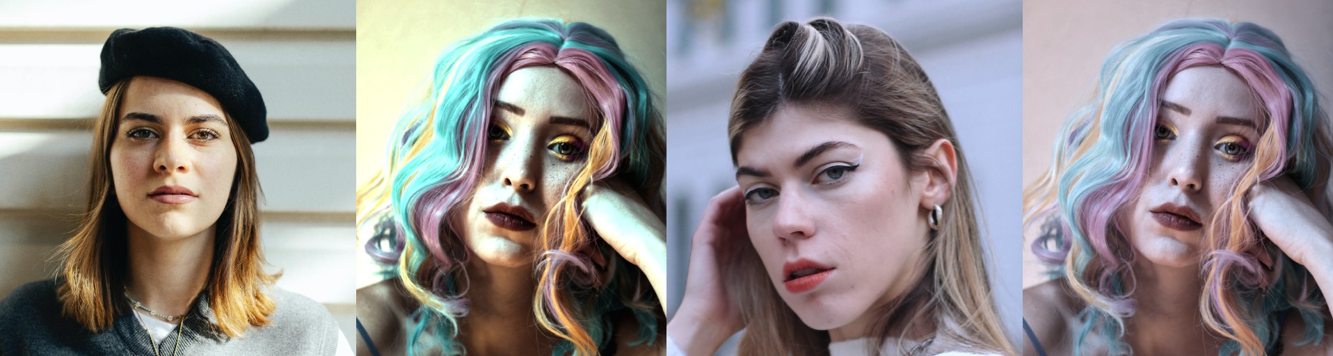
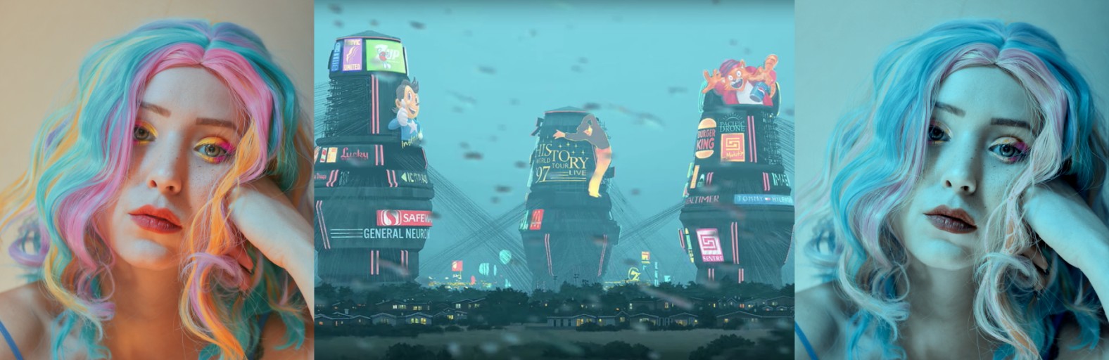
Fig. 16 Left: Highlights blown out because the optimizer doesn’t know the difference between faces and siding; Right: Image desaturated trying to match hair and background color (photographs by Esma Atak [4] and Sadettin Dogan [5] respectively)
Footnotes